Introduction
The basic algorithm for Gibbs Sampler is as follows.

From my understanding, there are two applications of Gibbs sampler as well as general Monte Carlo Markov Chain (MCMC) samplers.
The first application is to sample multivariable data point from a certain distributions, which is relatively easy.

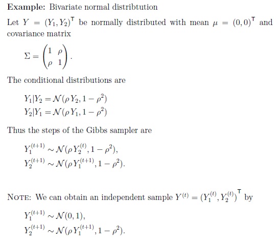
If you want to sample data from a bivariate normal distribtution, here is what you can do using Gibbs sampler.

The second application is to do Bayesian Inference of the parameters behind a certain dataset, which is relatively difficult to some extent, and requires more expertise in math. This is what I am going to emphasize on in this blog article.
Gibbs Sampler Inference
Here is a very good problem example of Gibbs Sampler Bayesian Inference. The author also provided the implementation code for solving the problem using Gibbs Sampler, which you could also download it here.
The original code is a little bit confusing, although it is correct. I rewrote and annotated it so that one can understand it more easily. You may download my code here.
# Gibbs sampler for the change-point model described in a Cognition cheat sheet titled "Gibbs sampling."
# This is a Python implementation of the procedure at http://www.cmpe.boun.edu.tr/courses/cmpe58n/fall2009/
# Written by Ilker Yildirim, September 2012.
# Revised and Annotated by Lei Mao, June 2017.
# dukeleimao@gmail.com

from scipy.stats import uniform, gamma, poisson
import matplotlib.pyplot as plt
import numpy
from numpy import log,exp
from numpy.random import multinomial

# fix the random seed for replicability.
numpy.random.seed(0)

# Generate data

# Hyperparameters
# Number of total data points
N=50

# Change-point: where the intensity parameter changes.
# The threhold point of two sets of data points
# n <= N
# Here we set n = 23
n=23
print str(n)

# Intensity values
# lambda1 for generating the first set of data from Poisson distribution
# Here we set lambda1 = 2
lambda1=2
# lambda2 for generating the second set of data from Poisson distribution
# Here we set lambda1 = 8
lambda2=8

# Generating observations x, consisting x_1 ... x_N
lambdas=[lambda1]*n
lambdas[n:N-1]=[lambda2]*(N-n)

x=poisson.rvs(lambdas)

# Make one big subplots and put everything in it.
f, (ax1,ax2,ax3,ax4,ax5)=plt.subplots(5,1)
# Plot the data
ax1.stem(range(N),x,linefmt='b-', markerfmt='bo')
ax1.plot(range(N),lambdas,'r--')
ax1.set_ylabel('Counts')

# Given the dataset, our mission is to model this dataset
# Our hypothesis is that the dataset consists two set of data, each set of the
# data satisfies Poisson distribution (You can also model the data using other
# distributions, say, Normal distribution, to see whether it works).
# We need to infer three parameters in the model using the dataset we have.
# 1. The threhold point of two sets of data points n
# 2. lambda1 for the first Poisson distribution dataset
# 3. lambda2 for the second Poisson distribution dataset

# Gibbs sampler
# Number of parameter sets we are going to sample
E=5200
# Number of parameter sets at the beginning of sampling we need to remove
# This is called "BURN-IN"
BURN_IN=200

# Initialize the chain
# Model n to be uniformly distributed from 0 to N
n=int(round(uniform.rvs()*N))
# Model lambda to satisfy gamma distribution
# We mannually set the gamma distribution parameter
a=2
b=0.2
lambda1=gamma.rvs(a,scale=1./b)
lambda2=gamma.rvs(a,scale=1./b)

# My understanding is that the model of these three variables should at least
# sample the true values of the variables with probablities larger than 0 (here
# the uniform distribution could sample variables from 0 to N, gamma
# distribution could sample variables greater or equal to 0), and the posterior
# conditionals of these three could be calculated easily using Bayesian
# Equations. Finally, this posterior probability distribution should be easy to
# use for sampling.

# Store the samples
chain_n=numpy.array([0.]*(E-BURN_IN))
chain_lambda1=numpy.array([0.]*(E-BURN_IN))
chain_lambda2=numpy.array([0.]*(E-BURN_IN))

for e in range(E):
	print "At iteration "+str(e)
	# sample lambda1 and lambda2 from their posterior conditionals, Equation 8 and Equation 9, respectively.
	lambda1=gamma.rvs(a+sum(x[0:n]), scale=1./(n+b))
	lambda2=gamma.rvs(a+sum(x[n:N]), scale=1./(N-n+b))

	# sample n, Equation 10
	mult_n=numpy.array([0]*N)
	for i in range(N):
		mult_n[i]=sum(x[0:i])*log(lambda1)-i*lambda1+sum(x[i:N])*log(lambda2)-(N-i)*lambda2
	mult_n=exp(mult_n-max(mult_n))
	n=numpy.where(multinomial(1,mult_n/sum(mult_n),size=1)==1)[1][0]

	# store
	if e>=BURN_IN:
		chain_n[e-BURN_IN]=n
		chain_lambda1[e-BURN_IN]=lambda1
		chain_lambda2[e-BURN_IN]=lambda2


ax2.plot(chain_lambda1,'b',chain_lambda2,'g')
ax2.set_ylabel('$\lambda$')
ax3.hist(chain_lambda1,20)
ax3.set_xlabel('$\lambda_1$')
ax3.set_xlim([0,12])
ax4.hist(chain_lambda2,20,color='g')
ax4.set_xlim([0,12])
ax4.set_xlabel('$\lambda_2$')
ax5.hist(chain_n,50)
ax5.set_xlabel('n')
ax5.set_xlim([1,50])
plt.show()
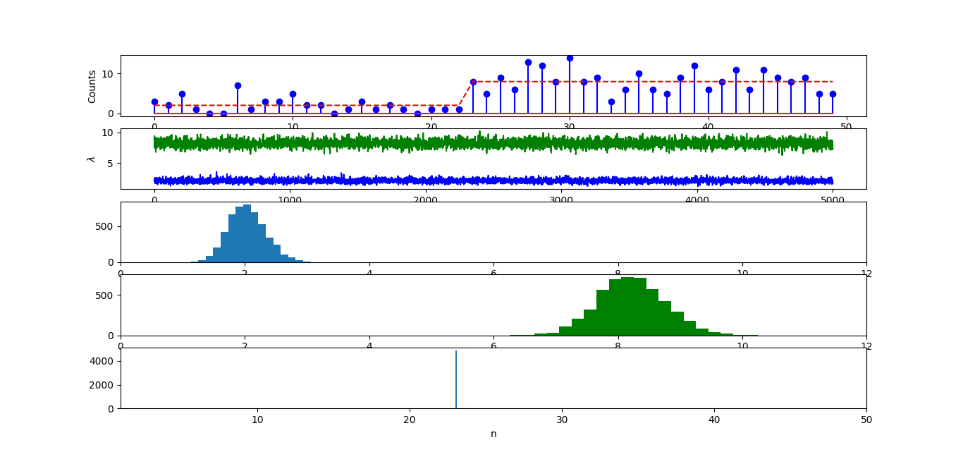
The output is as follows. The infered parameters matches the ones used for generating the data pretty well. The infered n equals exactly 23. The infered lambda1 and lambda2 were also centered at 2 and 8, respectively.

It should be noted that if you changed the parameters in the model (here, a and b for the gamma distribution), or even changed the model (say, uniform distribution to normal distribution, gamma distribution to normal distribution). The good infered parameters might not match the “real ones” exactly, but they should be very close.
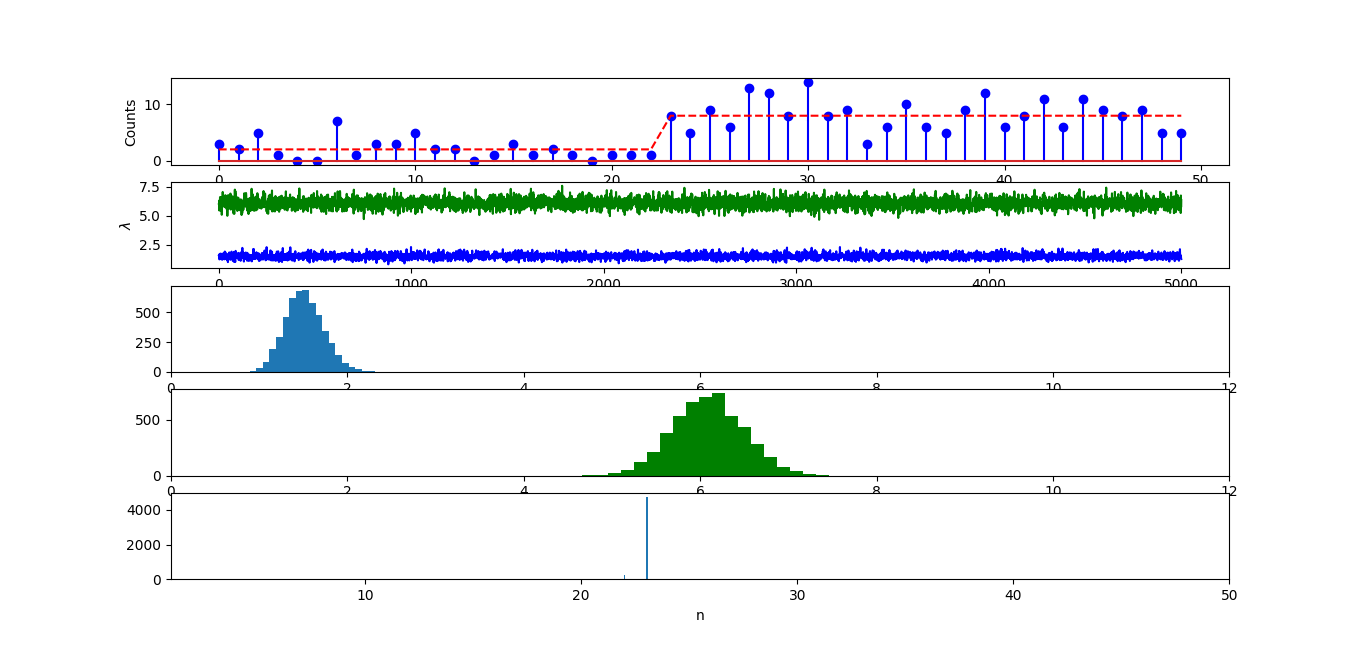
Here, if I change a from 2 to 5, change b from 0.2 to 10. The infered n equals around 23. However, the infered lambda1 and lambda2 were centered at 1.5 and 6, respectively. This is very bad, because for lambda2, the true value, which is 8, was not even sampled once.

So, how can we find there is a problem here, given we do not know the true parameters in real problems.
I have an idea but I am not sure whether this is correct in principle, or whether there is any theory to support this.
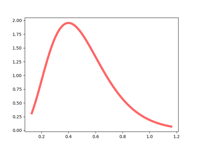
For a = 2, b = 0.2, the probability density function of gamma distribution (lambda1, lambda2 ~ Gamma(a = 2, b = 1/0.2)) is like this (click here to download the code for the probability density function plot of gamma distribution).

After Gibbs sampling, we know that the priors for lambda1 and lambda2 (lambda1 = 2, lambda2 = 8) are very high.
For a = 5, b = 10, the probability density function of gamma distribution (lambda1, lambda2 ~ Gamma(a = 5, b = 1/10)) is like this.

After Gibbs sampling, we know that the priors for lambda1 and lambda2 (lambda1 = 1.5, lambda2 = 6) are extremely low.
Although I am not sure whether there is any correlation between the prior probabilities and the “correctness of inference”, it should be noted that, even with the inference using a = 5 and b = 10, I can still reconstruct the dataset very well, which means that the choice of these model parameters might not have significant impact on our real studies.
