Introduction
Unlike other generative models, what’s interesting about the Generative Adversarial Networks (GANs) is that it is a combination of learning algorithm and game theory.

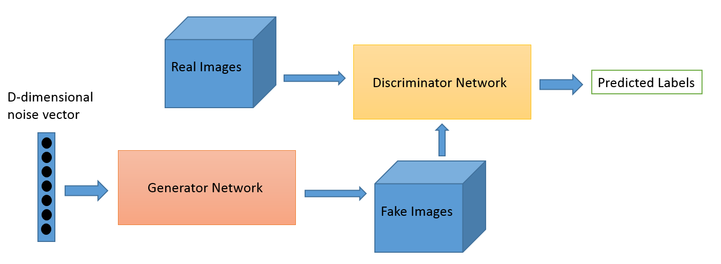
One of the typical GANs architeture is presented above. GANs have a generator network and discriminator network. Each of the generator netowrk and discriminator network has its own loss function. We are going to train these two neural networks simutaneously.
Here I am telling a metaphor about the GANs which I have heard from many sources. The generator is a conterfeiter who is trying to make fake money that looks like real. The discriminator is the police officer who is trying to identify if the money that the counterfeiter made along with other real money are real or fake. After each round of money counterfeiting and classification (training of our model), the conterfeiter and the police officer will be informed if the money that the conterfeiter made has been identified as real by the police officer. The police officer will also be informed if he has mis-classify any real money as fake. With this information (data label in our model), the counterfeiter will improve his skill in counterfeiting the money and the police officer will also improve his skill in classifying the real and fake money, until they reach the Nash Equilibrium which is a concept in Game Theory. This is actually a process of supervised learning.

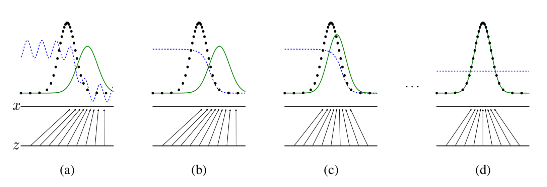
The above figure, which describes the game between the learnings of generator and discriminator, is taken from Ian Goodfellows’s 2014 GANs paper. $z$ is the random noise used to generate data in the latent space. $x$ is the data generated from $z$. The black curve is the true data distribution $p_{data}$. The green curve is the distribution of the data that the model generates $p_{model}$. The blue curve is the discriminator $D$, where optimally $D(x) = \frac{p_{data}(x)}{p_{data}(x) + p_{model}(x)}$. After learning for sufficient amount of time, the system reaches Nash Equilibrium (Figure (d)) where $p_{data} = p_{model}$ and $D(x) = 0.5$. In general, GANs are extremely difficult to train. Someone says even for this 1D case, it is difficult to reach this equilibrium as expected (Karpathy’s GANs Demo).
Materials
NIPS 2016 Tutorial: Generative Adversarial Networks
Ian Goodfellow’s 2-hour tutorial session covering some basic concepts and applications.
I had some problems understanding some part of the theory in the tutorial, such as the mathematical derivation. His 2014 GANs paper is a good auxilliary study material to the video tutorial.
Generative Adversarial Nets - Fresh Machine Learning #2
Siraj’s 5-miniute introduction to Generative Adversarial Networks. It is of course impossible to digest GANs in 5 minutes. Fortunately he provided a simple code demo to look at.
This GANs code demo generates 1D data.
He has also made a pokemon generator pokeGAN using GANs. Although the sample pokemon that GANs generated does not look “normal”, the code might be good for beginners to look at.
O’Reilly Tutorial on GANs
This is a hands-on GANs coding tutorial using TensorFlow. The source code can also be downloaded from my GitHub.
I read all the code. The code is overall good except for that it has some unexplained neural network architecture design.
For example, in the generator network, for the final convolution, its kernel/filter size is only [1, 1, z_dim/4] with a stride of 2 at each dimension to reduce the image size from [56, 56] to [28, 28]. The design of such kernel/filter will lose the useful information from the network. I would use [3, 3, z_dim/4] instead of [1, 1, z_dim/4].
def generator(z, batch_size, z_dim):
    g_w1 = tf.get_variable('g_w1', [z_dim, 3136], dtype=tf.float32, initializer=tf.truncated_normal_initializer(stddev=0.02))
    g_b1 = tf.get_variable('g_b1', [3136], initializer=tf.truncated_normal_initializer(stddev=0.02))
    g1 = tf.matmul(z, g_w1) + g_b1
    g1 = tf.reshape(g1, [-1, 56, 56, 1])
    g1 = tf.contrib.layers.batch_norm(g1, epsilon=1e-5, scope='bn1')
    g1 = tf.nn.relu(g1)

    # Generate 50 features
    g_w2 = tf.get_variable('g_w2', [3, 3, 1, z_dim/2], dtype=tf.float32, initializer=tf.truncated_normal_initializer(stddev=0.02))
    g_b2 = tf.get_variable('g_b2', [z_dim/2], initializer=tf.truncated_normal_initializer(stddev=0.02))
    g2 = tf.nn.conv2d(g1, g_w2, strides=[1, 2, 2, 1], padding='SAME')
    g2 = g2 + g_b2
    g2 = tf.contrib.layers.batch_norm(g2, epsilon=1e-5, scope='bn2')
    g2 = tf.nn.relu(g2)
    g2 = tf.image.resize_images(g2, [56, 56])

    # Generate 25 features
    g_w3 = tf.get_variable('g_w3', [3, 3, z_dim/2, z_dim/4], dtype=tf.float32, initializer=tf.truncated_normal_initializer(stddev=0.02))
    g_b3 = tf.get_variable('g_b3', [z_dim/4], initializer=tf.truncated_normal_initializer(stddev=0.02))
    g3 = tf.nn.conv2d(g2, g_w3, strides=[1, 2, 2, 1], padding='SAME')
    g3 = g3 + g_b3
    g3 = tf.contrib.layers.batch_norm(g3, epsilon=1e-5, scope='bn3')
    g3 = tf.nn.relu(g3)
    g3 = tf.image.resize_images(g3, [56, 56])

    # Final convolution with one output channel
    g_w4 = tf.get_variable('g_w4', [1, 1, z_dim/4, 1], dtype=tf.float32, initializer=tf.truncated_normal_initializer(stddev=0.02))
    g_b4 = tf.get_variable('g_b4', [1], initializer=tf.truncated_normal_initializer(stddev=0.02))
    g4 = tf.nn.conv2d(g3, g_w4, strides=[1, 2, 2, 1], padding='SAME')
    g4 = g4 + g_b4
    g4 = tf.sigmoid(g4)

    # Dimensions of g4: batch_size x 28 x 28 x 1
    return g4
